Generalized Linear Model
Modeling proportion/binary data
GLM for proportion/binary data
- Logistic regression is binomial glm with logistic links
- When to use binomial regression / quansi binomial regression / beta regression / beta binomial regression ?
Gamma regression
The parametrization of gamma distribution
- Gamma distribution commonly has two type of parametrization
- Shape \(\alpha\) and rate \(\beta\)
- Shape \(k\) and scale \(\theta\)
- Rate and shape follows \(\theta=1/\beta\)
- In GLM, the mean \(\mu = \alpha/\beta = \alpha\theta\) and shape \(\alpha\) parametrization was used
- The Gamma GLM in both R and python
statsmodelassume constant shape \(\alpha\), and inverse of \(\alpha\) is called dispersion \(\phi=1/\alpha\) - In
statsmodels,scalehas a distinct meaning, the estimated dispersion \(\phi=1/\alpha\) calledscale- The actual scale \(\theta\) can be calculated from model’s predicted mean \(\mu\)
- MASS package provide more precised estimation of the fixed shape patrameter
Simulate data
- In the following setting
- fixed shape \(\alpha=2\)
- intercept is 0.5
- cofficient is 0.8
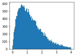
## Import packages import statsmodels.api as sm import matplotlib.pyplot as plt import scipy.stats as stats import numpy as np # Generate data np.random.seed(1) x=np.random.uniform(0,100,50000) mask = (x>50) x[mask],x[~mask] = 1,0 x2 = sm.add_constant(x) a,b = 0.5,0.8 y_true = a+b*x # Add error shape = 2 scale = y_true/shape y = np.random.gamma(shape=shape, scale=scale)- Histogram of simulated data
- Fit glm model
# Fit gamma glm with identity link function glm = sm.GLM(y, x2, family=sm.families.Gamma(sm.genmod.families.links.identity())) model = glm.fit() - The estimated shape parameter
1/model.scale # 1.9845020937600035 ~ 2 - Simulate data when covariate is 1 using the fitted parameters
- model.predict generate predicted \(\mu\)
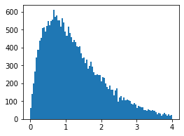
shape = 1/model.scale mean = model.predict(exog=np.array([[1,1]])) scale = mean/shape x1_pred = np.random.gamma(shape=shape, scale=scale,size=y[mask].shape[0])- Histogram of predicted data
Doing Similar Things in R
- Simulate data with known parameter and fit with GLM
  # Fit gamma glm with simulated data
  set.seed(1)
  x <- runif(50000, min = 0, max = 100)
  mask <- (x>50)
  x[mask] = 1;x[!mask] = 0
  a <- 0.5;b <- 0.8
  y_true <- a + b * x
  shape <- 2
  scale <- y_true/shape
  y <- rgamma(n = length(x), shape = shape, scale = scale)
  gamma.glm <- glm(y ~ x, family = Gamma(link = "identity"))

  # Cofficient in glm.summarized should nearly idetical to the simulation setting
  glm.summarized <- summary(gamma.glm)
  shape.hat.glm <- 1/glm.summarized$dispersion

  # MASS use MLE to get shape estimation claimed to be more accurate
  library(MASS)
  shape.hat.mass <- MASS::gamma.shape(gamma.glm)$alpha

  # Sampling data from fitted model
  N <- 1000
  rate <- shape.hat.mass/predict(gamma.glm,data.frame(x=c(1.3)))
  sampled <- rgamma(N,rate=rate,shape=shape.hat.mass)
Difference between Bernoulli vs. Binomial Response in logit model
-
See discussion here https://stats.stackexchange.com/questions/144121/logistic-regression-bernoulli-vs-binomial-response-variables
-
Link function for modeling proportion data
-
http://strata.uga.edu/8370/rtips/proportions.html
Statistical testing for methylation data
-
https://kkorthauer.org/fungeno2019/methylation/slides/1-intro-slides.html
- 2016, Bioinformatics, Differential methylation analysis for BS-seq data under general experimental design
-
R package DSS
- Also see 2016, BIB, Statistical method evaluation for differentially methylated CpGs in base resolution next-generation DNA sequencing data
Reference
- https://stackoverflow.com/questions/64174603/how-to-use-scale-and-shape-parameters-of-gamma-glm-in-statsmodels
- https://stats.stackexchange.com/questions/247624/dispersion-parameter-for-gamma-family
- https://stackoverflow.com/questions/60215085/calculating-scale-dispersion-of-gamma-glm-using-statsmodels
- https://en.wikipedia.org/wiki/Gamma_distribution