PCA, CCA and ICA
- Three related dimensional reduction technique with application in gene expression data analysis
- PCA: principle component analysis
- CCA: canonical correlation analysis
-
ICA: individual components analysis
- Consider we have a gene expression matrix, rows are genes, columns are samples
PCA
- A linear projection that maximize variations or minimize reconstruction loss
- Suppose we have \(N\) samples, \(X_1\),\(X_2\),…,\(X_n\), each samples is a \(d\) dimensional vector
- Sample mean is: \(\bar{X}=\frac{\sum_{1}^{n}X_{i}}{N}\)
- Given a projection vector \(u_1\) with dimension \(d\), the projected vector is \(\hat{X_i} = u_{1}^TX_i\)
- Mean of projected vector is \(\frac{\sum_{1}^{n}\hat{X_{i}}}{N} = \frac{\sum_{1}^{n}u_{1}^TX_i}{N} = u_{1}^T\bar{X}\)
The projected variance maximization formulation
- Variance of projected vector is:
-
Where \(S=\frac{1}{N} \sum_{1}^{n}(X_i - \bar{X})(X_i - \bar{X})^T\) is the covariance matrix
-
Here we want to maximize \(u_{1}^TSu_{1}\)
-
We add a restrain \(u_{1}^Tu_{1}=1\)
-
We have the language multiplier:
- Take the derivitive, we have
-
Hence the projection that maximize variance of projected vector is the eigen vector corresponds to the largest eigen value
-
As \(S^H=S\), \(S\) is a Hermitian matrix (埃米尔特矩阵)
-
Hermitian matrix has orthogonal eigenvectors for distinct eigenvalues
-
Other eigen vector with smaller eigen values are other projections orthogonal to \(u_1\)
Reference
CCA
- Given two random vectors \(X\) and \(Y\), CCA seeks for two linear combination of these vectors, to maximize their correlation
Applications in cross studies and cross species integration of transcriptomic profile
- An implementation for strategy used in Integrating single-cell transcriptomic data across different conditions, technologies, and species (2018,NBT)
- Load TCGA CRC tumor / normal tissue data
import pandas as pd
import numpy as np
from matplotlib import pyplot as plt
import seaborn as sns
from sklearn.decomposition import PCA
from sklearn.cross_decomposition import CCA
from sklearn.preprocessing import StandardScaler

# Normalize and scale expression matrix
def tranform(matrix):
    CPM = matrix/matrix.sum(axis=0).values.reshape(1,-1)
    CPM = np.log(CPM+1)
    X = StandardScaler().fit_transform(CPM.T.values)
    return pd.DataFrame(data = X.T,index = CPM.index,columns=CPM.columns)

CRC_home = pd.read_csv("data/CRC-home.txt",sep="\t",index_col=0)
CRC_TCGA = pd.read_csv("data/CRC-TCGA.txt",sep="\t",index_col=0)
merged_ids = np.intersect1d(CRC_home.index,CRC_TCGA.index)
CRC_merged = CRC_home.loc[merged_ids,:].join(CRC_TCGA.loc[merged_ids,:])
CRC_TCGA_scaled = tranform(CRC_TCGA)
CRC_home_scaled = tranform(CRC_home)
CRC_merged_scaled = tranform(CRC_merged)
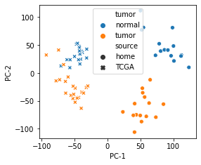
- Show batch effect in different studies with PCA (other dimensional reduction techniques will also work)
- As shown in figure bellow, sample of same tissue in different studies is quiet distinctive
CRC_merged_X2 = PCA(n_components=2).fit_transform(CRC_merged_scaled.values.T)
CRC_merged_table = pd.DataFrame(data=CRC_merged_X2,index=CRC_merged_scaled.columns,columns=["PC-1","PC-2"])
CRC_merged_table["tumor"] = CRC_merged_scaled.columns.map(lambda x:"normal" if x.endswith("N") or x.split("-")[-1]=="11A" else "tumor")
CRC_merged_table["source"] = CRC_merged_table.index.map(lambda x:"home" if x.startswith("CRC") else "TCGA")
fig,ax = plt.subplots(figsize=(4,3.5))
g = sns.scatterplot(data=CRC_merged_table,x="PC-1",y="PC-2",hue="tumor",style="source")
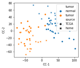
- Use CCA to super-impose similar cell types in different studies
- Convert scaled gene expression matrix to gene loading matrix with CCA
- k conanical components
- Consider \(n\) genes in dataset \(X\) and \(Y\), \(p\) sample in \(X\), \(q\) sample in \(Y\)
- Convert gene expression matrices \(X_{n,p}\) \(Y_{n,q}\) to gene loading matrices \(A_{n,k}\) \(B_{n,k}\)
-
Perform QR decomposition on gene loading matrix
\[A_{n,k}=D_{n,k}R_{k,k}\] \[B_{n,k}=E_{n,k}R_{k,k}\] - Calculate the projected matrix
- Map gene points to sample points
- Convert scaled gene expression matrix to gene loading matrix with CCA
# Convert scaled gene expression matrix to gene loading matrix with CCA
cca = CCA(n_components=10).fit(CRC_home_scaled.loc[merged_ids,:].values,CRC_TCGA_scaled.loc[merged_ids,:].values)
home_CC,TCGA_CC = cca.transform(CRC_home_scaled.loc[merged_ids,:].values,CRC_TCGA_scaled.loc[merged_ids,:].values)

# Perform **QR** decomposition on gene loading matrix
TCGA_CC_Q,TCGA_CC_R = np.linalg.qr(TCGA_CC)
home_CC_Q,home_CC_R = np.linalg.qr(home_CC)

# Calculate the projected matrix
CRC_TCGA_scaled_projected = np.dot(CRC_TCGA_scaled.loc[merged_ids,:].values.T,TCGA_CC_Q)
CRC_home_scaled_projected = np.dot(CRC_home_scaled.loc[merged_ids,:].values.T,home_CC_Q)

# Visualize
TCGA_scaled_projected_table = pd.DataFrame(data = CRC_TCGA_scaled_projected[:,:3],index = CRC_TCGA_scaled.columns,columns = ["CC-1","CC-2","CC-3"])
home_scaled_projected_table = pd.DataFrame(data = CRC_home_scaled_projected[:,:3],index = CRC_home_scaled.columns,columns = ["CC-1","CC-2","CC-3"])
TCGA_scaled_projected_table["tumor"] = CRC_TCGA.columns.map(lambda x:"normal" if x.split("-")[-1]=="11A" else "tumor")
TCGA_scaled_projected_table["source"] = "TCGA"
home_scaled_projected_table["tumor"] = CRC_home.columns.map(lambda x:"normal" if x.endswith("N") else "tumor")
home_scaled_projected_table["source"] = "home"
CRC_scaled_projected_table = pd.concat([TCGA_scaled_projected_table,home_scaled_projected_table])
fig,ax = plt.subplots(figsize=(4,3.5))
sns.scatterplot(data=CRC_scaled_projected_table,x="CC-1",y="CC-2",style="source",hue="tumor")
plt.savefig("CCA-CRC-tissue.png",bbox_inches="tight")
Some tools
Some tutorial
ICA
- Independent Component Analysis:Algorithms and Applications
- An informationmaximisation approach to blind separation and blind deconvolution
- Blind source separation
- A mixture of signal, don’t known the source
- Based on the assumption that any two signal is independent
- The fundamental restriction in ICA is that the independent components must be nongaussian for ICA to be possible.
- Note uncorrelated random variable are not always independent