Regularization to Incorporate Structure Information
有时你会希望在预测模型中加入一些先验的结构信息。
比方说你用LASSO做特征选择。你的特征是一段基因组上每个位点的数值,你希望相邻的两个位点能以比较大的概率被同时选中。或者你的特征是一些基因的表达量,你先验的知道一些基因共表达的信息,你希望共表达的基因尽可能的同时被选中。或者你想用NMF对一个基因表达的矩阵进行降维。这时候你可能希望已知被共调控的基因被在降维后处在比较接近的位置。像这种情况都可以在正则化上做文章。
Generalized Regularization in LASSO regression
对于第一个基因组位点选择的例子,有人提出了一种叫做fused LASSO的做法,见https://web.stanford.edu/group/SOL/papers/fused-lasso-JRSSB.pdf。假设我们有从标号为从1到p的连续排列的p个特征,那么fused LASSO的loss可以定义成:
\[L(\beta,\lambda_{1},\lambda_{2}) = \frac{1}{2} (y-X\beta)^T(y-X\beta) + \lambda_{1}\sum_{j=1}^{p}|\beta_{j}| + \lambda_{2}\sum_{j=2}^{p}|\beta_{j}-\beta_{j-1}|\]如果想同时选中先验的认为比较相近的特征,有两种非常相似的方法,一种叫做grouped LASSO, 还有一种叫做graph regularized LASSO。
Group LASSO发表在http://pages.stat.wisc.edu/~myuan/papers/glasso.final.pdf。在grouped LASSO中, 假设特征被预先分成了从\(1\)到\(J\)的\(J\)组,其中第\(g\)组有\(p_{g}\)个特征,则loss被定义成:
\[L(\beta,\lambda) = \frac{1}{2} (y-X\beta)^T(y-X\beta) + \lambda\sum_{g=1}^{J}\sqrt{\beta_{g}^{T}\beta_{g}}\]另一种是graph regularized LASSO,见 https://academic.oup.com/bioinformatics/article/24/9/1175/206444。假设每一个特征之间的关系可以用一个图来表示,图上的每一个节点都对应着一个特征。假设\(A\)是图的邻接矩阵。所以每一个节点的度(degree)是:
\[d_{i} = \sum_{i}^{p}A_{i,j}\]所有节点的度可以表示为一个度数矩阵:
\[D = diag(d_{1},...,d_{i},...,d_{p})\]该图的拉普拉斯矩阵定义为:
\[L = D - A\]归一化的拉普拉斯矩阵为:
\(L^{sym} = D^{-\frac{1}{2}}LD^{-\frac{1}{2}} = I - D^{-\frac{1}{2}}AD^{-\frac{1}{2}}\)
这样loss可以定义成:
\[L(\beta,\lambda_{1},\lambda_{2}) = \frac{1}{2} (y-X\beta)^T(y-X\beta) + \lambda_{1}\sum_{j=1}^{p}|\beta_{j}| + \lambda_{2}\beta^TL^{sym}\beta\]这里比较迷惑的是凭什么\(\beta^TL^{sym}\beta\)就能作为一项正则化。实际上我们是希望图中有连接的节点系数都比较接近。 所以我们希望这样一个量是比较小的:
\[\frac{1}{2}\sum_{i=1}^{p}\sum_{j=1}^{p}A_{i,j}(\beta_{i}-\beta_{j})^{2}\]经过简单的计算不难发现:
\[\frac{1}{2}\sum_{i=1}^{p}\sum_{j=1}^{p}A_{i,j}(\beta_{i}-\beta_{j})^{2} = \sum_{i=1}^{p}\beta_{i}^2d_{i,i} - \sum_{i=1}^{p}\sum_{j=1}^{p}A_{i,j}\beta_{i}\beta_{j} = \beta^TD\beta - \beta^TA\beta = \beta^T(D-A)\beta\]如果考虑一个按度数归一化的版本:
\[\frac{1}{2}\sum_{i=1}^{p}\sum_{j=1}^{p}A_{i,j}(\frac{\beta_{i}}{\sqrt{d_{i}}}-\frac{\beta_{j}}{\sqrt{d_{j}}})^{2} = \beta^TL^{sym}\beta\]A implementation for fused LASSO in python
- Import reuiqred package
import numpy as np
import cvxpy
from matplotlib import pyplot as plt
from sklearn.decomposition import PCA
from sklearn.linear_model import LogisticRegression
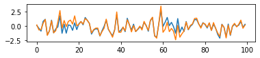
- Simulate artificial data. In this setting, in 100 features, features[10:20]和feature[60:70] are informative for distinguishing two class from each other
coff0 = np.random.randn(100)
coff1 = coff0 + np.random.randn(coff0.shape[0])*0.2
coff1[10:20] += 1
coff1[60:70] -= 1
def simulate_data(coff,n=100):
    X = np.random.randn(n,coff.shape[0])
    return 2*X + coff.reshape(1,-1)
X0 = simulate_data(coff0)
X1 = simulate_data(coff1)
y = np.concatenate([np.zeros(100),np.ones(100)])
X = np.concatenate([X0,X1],axis=0)
- Ilustrate simulated cofficients
fig,ax = plt.subplots(figsize=(6,1))
ax.plot(coff0)
ax.plot(coff1)
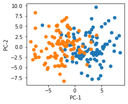
- Visualization simulated data with PCA
fig,ax = plt.subplots(figsize=(3.5,3))
X2d = PCA(n_components=2).fit_transform(X)
ax.scatter(X2d[:100,0],X2d[:100,1])
ax.scatter(X2d[100:,0],X2d[100:,1])
ax.set_xlabel("PC-1")
ax.set_ylabel("PC-2")
plt.savefig("2021-06-13-LR-PCA.png",bbox_inches="tight")
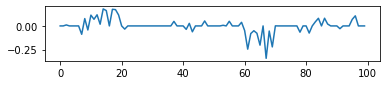
- Result of default LASSO in sklearn
logit_model = LogisticRegression(penalty="l1",solver='liblinear',C=0.1).fit(X,y)
fig,ax = plt.subplots(figsize=(6,1))
_ = ax.plot(logit_model.coef_.reshape(-1))
- Calculate three regularization terms
beta = cvxpy.Variable(100)
lambd = cvxpy.Parameter(nonneg=True)
lambd.value = 1
log_likelihood = cvxpy.sum(cvxpy.multiply(y, X @ beta) - cvxpy.logistic(X @ beta))
# L1 loss
l1_loss = cvxpy.norm(beta, 1)

# Soomthing loss
smooth_mat = np.zeros((beta.shape[0]-1,beta.shape[0]))
diag_indices = np.arange(smooth_mat.shape[0])
smooth_mat[(diag_indices,diag_indices)] = -1
smooth_mat[(diag_indices,diag_indices+1)] = 1
smooth_loss = cvxpy.norm(smooth_mat@beta, 1)
- Result of LASSO penalty alone
reg_term = 0.05*l1_loss
problem = cvxpy.Problem(cvxpy.Minimize(-log_likelihood/y.shape[0] + reg_term))
_ = problem.solve()
fig,ax = plt.subplots(figsize=(6,1))
_ = ax.plot(beta.value)
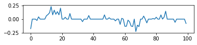
- Result of fused LASSO
reg_term = 0.05*l1_loss + 0.5*smooth_loss
problem = cvxpy.Problem(cvxpy.Minimize(-log_likelihood/y.shape[0] + reg_term))
_ = problem.solve()
fig,ax = plt.subplots(figsize=(6,1))
_ = ax.plot(beta.value)
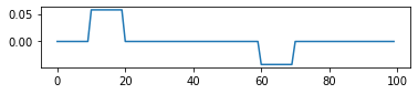
- We can see fused LASSO perfectly recovery the informative features (although this example is very artificial).
Regularization in NMF decomposition
- Frobenius norm
- NMF的正则化. See https://scikit-learn.org/stable/modules/generated/sklearn.decomposition.NMF.html
- 也可以用绝对值的和做正则化
- 在正则化中加入graph的信息
- https://academic.oup.com/bioinformatics/article/34/2/239/4101940
- 例如我们有一个表达矩阵\(Y_{n,m}\),有一个图\(G^{gene}\)来描述基因间的关系,有一个图\(G^{sample}\)来描述样本间的相似性
- 我们希望分解出\(W_{n,k}\)和\(H_{m,k}\)两个矩阵分别反应基因和样本的信息
- \(G^{gene}\)的Graph Laplacian为\(L_{gene}\), \(G^{sample}\)的Graph Laplacian为\(L_{sample}\),
- 还有一些用图的正则化做非负矩阵分解的例子,见https://www.nature.com/articles/nmeth.2651和https://ieeexplore.ieee.org/document/5674058。
Further Reading
- http://www.stat.cmu.edu/~ryantibs/papers/genlasso.pdf
- http://euler.stat.yale.edu/~tba3/stat612/lectures/lec22/lecture22.pdf
- Read this book https://web.stanford.edu/~hastie/StatLearnSparsity/ for more technical discussion