Probablistic Model for Sequence Analysis
- 看了不知道多少遍总是记不清楚,详细记录一下,希望别再忘了:)
EM algorithm for motif finding
- Input data: \(n\) sequences \(X_1,X_2,...,X_n\) with different lengths
- Find ungapped motif with fixed length \(w\)
- \(\theta\) is the motif paramter and background paramater
- There are \(m_i=L_i-w+1\) possible staring position in sequence \(X_i\) with length \(L_i\)
- \(Z_{ij}\) is a binary indicator variable, indicate whether there is a motif start at position \(j\) in sequence \(i\)
- Denote number of motifs in sequence \(i\) as \(Q_i=\sum_{j=1}^{m_i}Z_{ij}\).
- A sequence may contains 0 motifs, 1 motifs or more than one motifs.
OOPS
-
assume one occurrence per sequence
-
Likelihood of a sequence given the motif position
- Prior probability that \(Z_{ij}=1\) (motif in sequence \(i\) starts at \(j\))
- Joint likelihood of sequence and motif start pisition for each seuence
- Joint log likelihood for each seuence
- EM for motif finding. Denote model paramters at step \(t\) as \(\theta^{(t)}\) s
- E step: calculate \(\mathbb{E}_{Z_{ij} \mid X_i,\theta^{(t)}} Z_{ij}\),
- M step: replace \(Z_{ij}\) in \(\log P(X_i,Z_i \mid \theta)\) with \(\mathbb{E}_{Z_{ij} \mid X_i,\theta^{(t)}} Z_{ij}\), perform standard MLE to update \(\theta^{(t)}\) to \(\theta^{(t+1)}\)
ZOOPS
-
assume zero or one motif occurrences per dataset sequence), add parameter \(\gamma\), probability that a sequence contains a motif. \(\lambda_i=\frac{\gamma}{m_i}\) is prior probabaility that any position in a sequence is start of a motif
-
Likelihood of a sequence contain one motif, given the motif position is same as OOPS
-
Likelihood of a sequence without a motif
- Joint likelihood of sequence and motif start pisition for each seuence
- Joint log-likelihood
-
EM for motif finding
-
E step: calculate \(\mathbb{E}_{Z_{ij} \mid X_i,\theta^{(t)}} Z_{ij}\)
TCM
-
two component mixture, motif can start at any feasible positions
-
Joint likelihood of sequence and motif start pisition for each seuence \(\begin{align*} P(X_i,Z_i|\theta,\lambda)&=P(X_i,Z_i|\theta,\lambda)\\ &=\prod_{j=1}^{m_i}\lambda^{Z_{ij}}(1-\lambda)^{1-Z_{ij}}P(X_{ij} \mid Z_{ij}=1)^{Z_{ij}}P(X_{ij} \mid Z_{ij}=0)^{1-Z_{ij}} \end{align*}\)
-
Joint log-likelihood \(\begin{align*} \log P(X_i,Z_i|\theta,\lambda) = \sum_{j=1}^{m} [Z_{ij} \log \lambda +(1- Z_{ij}) \log (1-\lambda) + (1-Z_{ij}) \log P(X_{ij} \mid Z_{ij}=0) + Z_{ij} \log P(X_{ij} \mid Z_{ij}=1)] \end{align*}\)
HMM
-
\(N\) is length of the observation
-
\(n\) is number of hidden states
-
Hidden state \(Q\):
- Emitted symbol \(O\):
-
Transition probability matrix \(A_{N \times N}\). \(a_{st} = A_{st}\) is transition probability from state \(s\) to \(t\)
\[a_{st} = P(q_{i}=t \mid q_{i-1}=s)\] -
Initial probability distribution of hidden states \(\pi\) or transition probability from a slilent starting state to state \(p_i\)
- Probability of emitting symbol \(b\) at state \(k\)
Forward algorithm (inference)
- Determine the likelihood of an observed series, marginalized for all possible hidden states
- Define the forward variable \(\alpha_{t}(j)\), that is given model parameter, the joint probability of being state \(j\) at time \(t\) with observation series \(o_1,o_2,...,o_t\)
- We have (\(\lambda\) is omitted)
- Initialization
- \(\alpha_{t}(j)\) can be determined by dynamic programming
- Marginalize across last hidden state
Viterbi algorithm (decoding)
-
Find the most probable path of hidden states, given the model and observation
-
Define the Viterbi variable
- The intialization is same as forward algorithm
- A dynamic programming similar to forward algorithm (the difference is replace \(\sum\) operator with \(\max\) operator) is used to calculate viterbi variable
- Keep track of the “best” hidden state, main a backtrace pointer matrix
Model training
- Estimation HMM parameter from observations
Baum–Welch algorithm: forward-backward algorithm based, EM style training
- Define backward variable \(\beta_{t}(i)\)
- Similar to forward variable, we have
-
We can use backward algorithm as an alternative to forward algorithm for calculating \(P(O \mid \lambda)\)
-
Initialization (last observation in each instance always transit to ending state with probability 1 regardless of the hidden state \(q_T\))
- Recursion
- Termination (exact same as the recursion fumula if we add a silent starting state corresponds to \(t=0\))
- The forward-backward algorithm
- To compute such expectation, we define a forward-backward variable
- Note
- Hence
Profile HMM
-
A spacial HMM primarily used for protein homolog modeling
- The hidden states in a profile HMM for local alignment, with N key positions
- start state
- insertion state 0, modeling left flanking background sequence
- match state at key position 1, insertion state at key position 1, deletion state at key position 1
- …
- match state at key position N, insertion state at key position N (modeling right flanking background sequence), deletion state at key position N
- end state
- Possible transitions
- begin \(\Rightarrow\) insertion state 0
- begin \(\Rightarrow\) deletion state at key position 1 (allow condition when first residue is missing)
-
begin \(\Rightarrow\) match state at key position 1
- insertion state 0 \(\Rightarrow\) insertion state 0
- self looping for left flanking background sequence modeling
- The looping probability on the flanking states should be close to 1, since they must account for long stretches of sequence
- insertion state 0 \(\Rightarrow\) deletion state at key position 1
-
insertion state 0 \(\Rightarrow\) match state at key position 1
- match state at key position i-1 \(\Rightarrow\) match state at key position i
- insertion state at key position i-1 \(\Rightarrow\) match state at key position i
-
deletion state at key position i-1 \(\Rightarrow\) match state at key position i
- match state at key position i-1 \(\Rightarrow\) deletion state at key position i
- insertion state at key position i-1 \(\Rightarrow\) deletion state at key position i
-
deletion state at key position i-1 \(\Rightarrow\) deletion state at key position i
- match state at key position i \(\Rightarrow\) insertion state at key position i
- insertion state at key position i \(\Rightarrow\) insertion state at key position i
- deletion state at key position i \(\Rightarrow\) insertion state at key position i
- “We have added transitions between insert and delete states, as they did, although these are usually very improbable. Leaving them out has negligible effect on scoring a match, but can create problems when building the model from MSA”
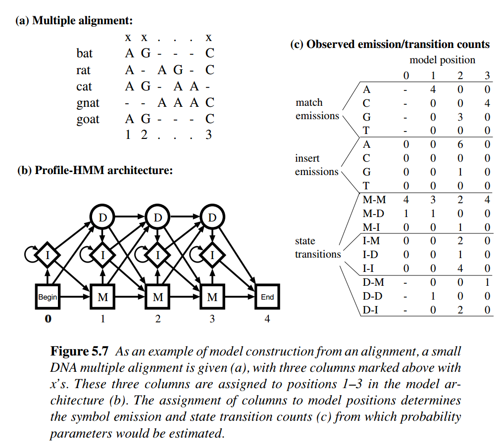
- In most cases, profile HMM is constructed from MSA. Consider Figure 5.7 in Biological Sequence Analysis. We can see given a column assignment for MSA, the \(D_i \Rightarrow I_i\) transition could occur
- match state at key position i \(\Rightarrow\) end
- insertion state at key position i \(\Rightarrow\) end
- self looping for right flanking background sequence modeling, should be close to 1
-
deletion state at key position i \(\Rightarrow\) end
- HMM Profile searching
- Viterbi algorithm and forward algorithm can both be used for HMM profiling searching
- Viterbi: assign a mostly likely hidden state for each nucleotide, and report the corresponding likelihood
- Viterbi variable for matching, insertion and deletion states at key position j and sequence position i
-
forward: assign a likelihood that the input sequence is generated from a HMM profile
-
See https://notebook.community/jmschrei/pomegranate/tutorials/B_Model_Tutorial_3_Hidden_Markov_Models
Model construction
- To construct profile HMM from MSA, we have to make a decision. Each column in the MSA should either be assigned to a key position (marked column), or an insertion (unmarked column).
- For columns marked as key positions, residues are assigned to match state, gaps are assigned to deletion state
- For columns marked as insertions, residues are assigned to insertions, gaps are ignored
- There are \(2^L\) ways to mark a MSA with \(L\) columns.
- Three ways for marking MSA columns
- Manual
- Heuristics: rule based assignment. For example, assigning all columns will more than a certain fraction of gap characters to insert states
- MAP (maximum a posteriori)