Notes on Markov Random Field
Notes on Markov Random Field
Definition and parameterization
- Markov random field is an undirectional probablistic graph model
- Consider random variables \(X=(X_1,X_2,...,X_n)\)
- These random variables have conditional dependency defined by a graph \(G\)
- The graph \(G\) have \(m\) cliques (fully connected subgraphs), denoted as \(D_1,...,D_m\)
- Then distribution of the random variable can be expressed as product of clique potentials:
- \(\phi_{i}(D_i)\) is potential of clique \(D_i\)
- \(Z\) is called partition function
-
Calculation of \(Z\) is generally computationally intractable
-
It can also expressed as an log-linear model
- \(w_{i}\) are weights
- \(f_{i}(D_{i})\) is the feature of complete subgraph \(D_{i}\)
- \(Z\) is the normalization constant, or partition function
Image denoising
Image segmentation
Ising / Potts model and protein / RNA contact prediction
Ising model
- Random variable \(X_i\) takes value of either 1 or -1
- The energy of edge (i,j) is
- The energy of variable \(X_i\) is
- The distribution takes the form
Potts model and protein / RNA structure modeling
- A protein sequence in multiple sequence alignment: \((\sigma_1,\sigma_2,\sigma_3,...,\sigma_N)\)
-
\(\sigma_1\) takes value from the protein/RNA alphabet and gap “-“
- mfDCA (mean field direct coupling analysis)
- plmDCA (pseudolikelihood maximization direct coupling analysis)
Restricted bolzmann machine
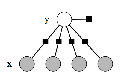
Conditional random field
- Direct modeling the conditional distribution \(P(y\|X)\), that is given observations of a subset of variables \(X\), modeling the distribution remaining variables \(Y\) conditioned on \(X\)
- Combining the advantages of discriminative classification and graphical modeling
- Combining the ability to compactly model multivariate outputs y with the ability to leverage a large number of input features x for prediction
-
Note \(X\) is not involved in calculation of partition function
-
Logistic regression is a special case of conditional random field
- It takes a form same as log-linear model of markov random field